Basic Graphical Methods for Time Series

library(forecast)
library(lubridate)

data("AirPassengers")

## Plot of Air Passengers with increasing variance
plot(AirPassengers, main = "Air Passengers 1949 to 1961", ylab = "Passengers")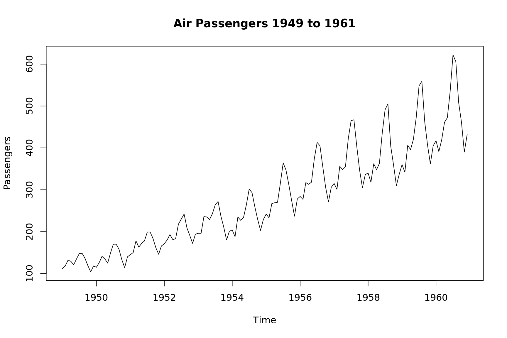

## Seasonal plot by year
seasonplot(AirPassengers, s = 12, main = "Seasonal Plot", ylab = "Passengers", year.labels = TRUE, col = 1:12)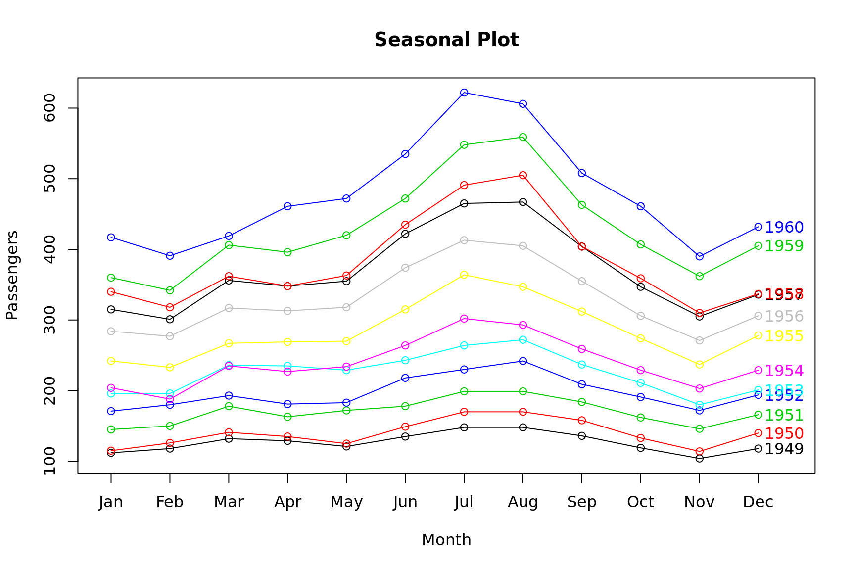

## Seasonal subseries plot
monthplot(AirPassengers, ylab = "Passengers", main = "Seasonal Deviation", labels = month.abb)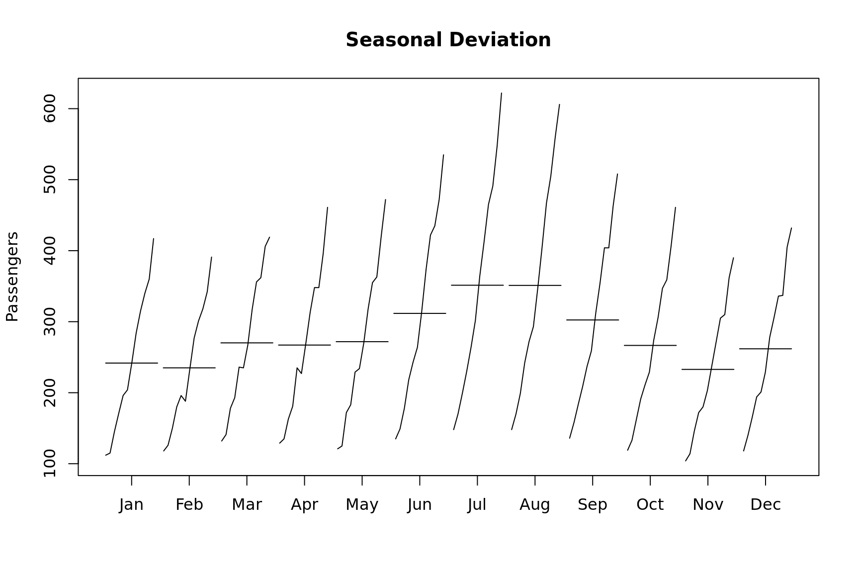

## Autocorrelation
acf(AirPassengers, main = "Autocorrelation")

Simple Forecasting Methods

## Average Method
method.avg = meanf(AirPassengers, h = 36)

## Naive Method
method.naive = naive(AirPassengers, h = 36)

## Seasonal Naive
method.snaive = snaive(AirPassengers, h = 36)

## Random Walk with Drift
method.rwf = rwf(AirPassengers, h = 36, drift = TRUE)

## Plot of the different methods
plot(AirPassengers, main = "Air Passengers 1949 to 1961", xlim = c(1949, 1964))
lines(method.avg$mean, col = 2)
lines(method.naive$mean, col = 3)
lines(method.snaive$mean, col = 4)
lines(method.rwf$mean, col = 5)
legend("topleft", lty = 1, col = c(2, 3, 4, 5),
       legend = c("Average", "Naive", "Seasonal Naive", "Random Walk"))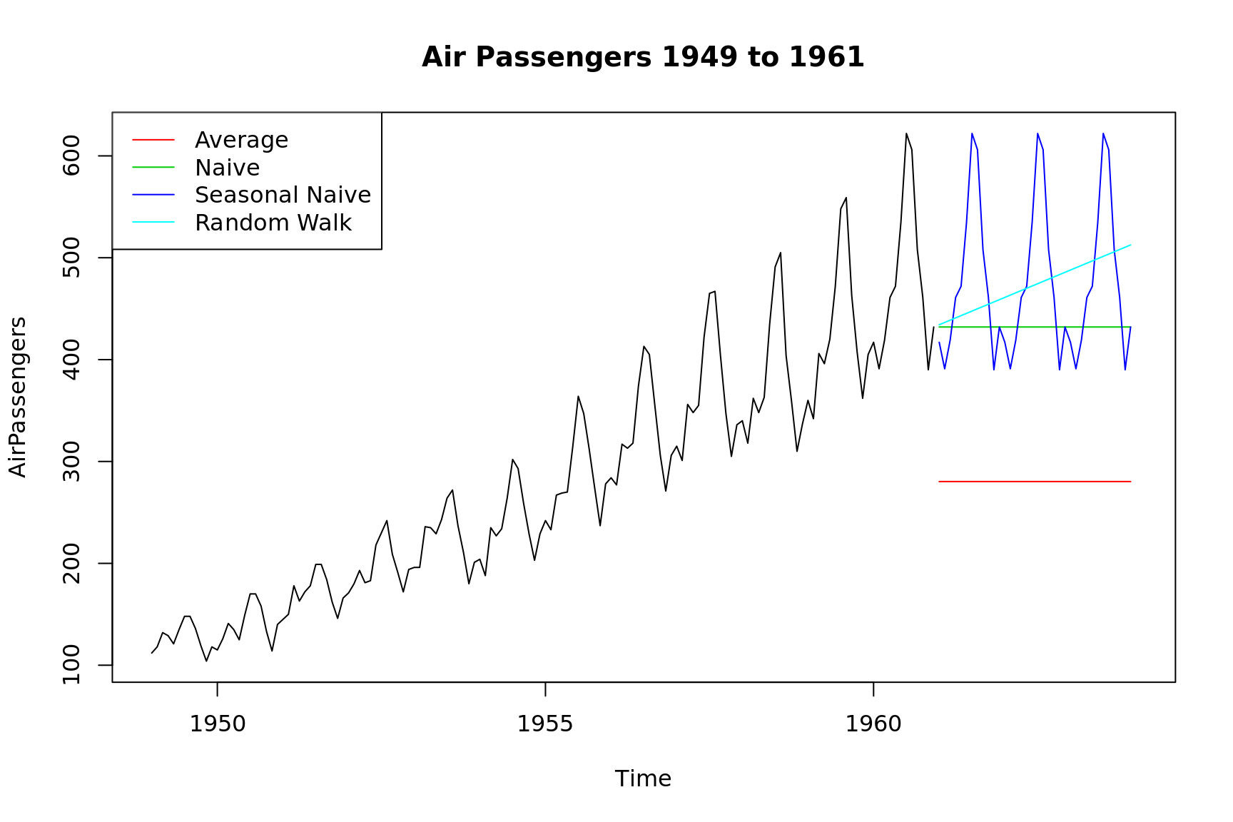

Stabalizing Variance

## Box Cox Transformation
(lambda = BoxCox.lambda(AirPassengers))

[1] -0.2947156

## Remove variation from months, create a data.frame first
Air = data.frame(Passengers = AirPassengers)
Air$Date = seq.Date(from = as.Date("1949-01-01"), by = "month", length.out = 144)

## Calculate days per month
Air$Days.per.month = days_in_month(Air$Date)

## Calculate average number of passengers per month removing variation due to number of days
Air$month.avg = with(Air, Passengers / Days.per.month)

## Plots of original data and monthly average under the Box Cox Transformation
par(mfrow = c(2, 1))
plot(BoxCox(Air$Passengers, lambda), ylab = "Passengers", main = "Air Passengers (BCT)")
plot(BoxCox(Air$month.avg, BoxCox.lambda(Air$month.avg)), ylab = "Passengers",
     main = "Passengers Per Month (BCT)")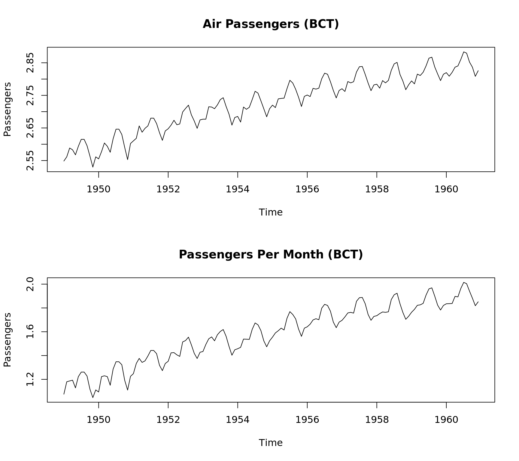

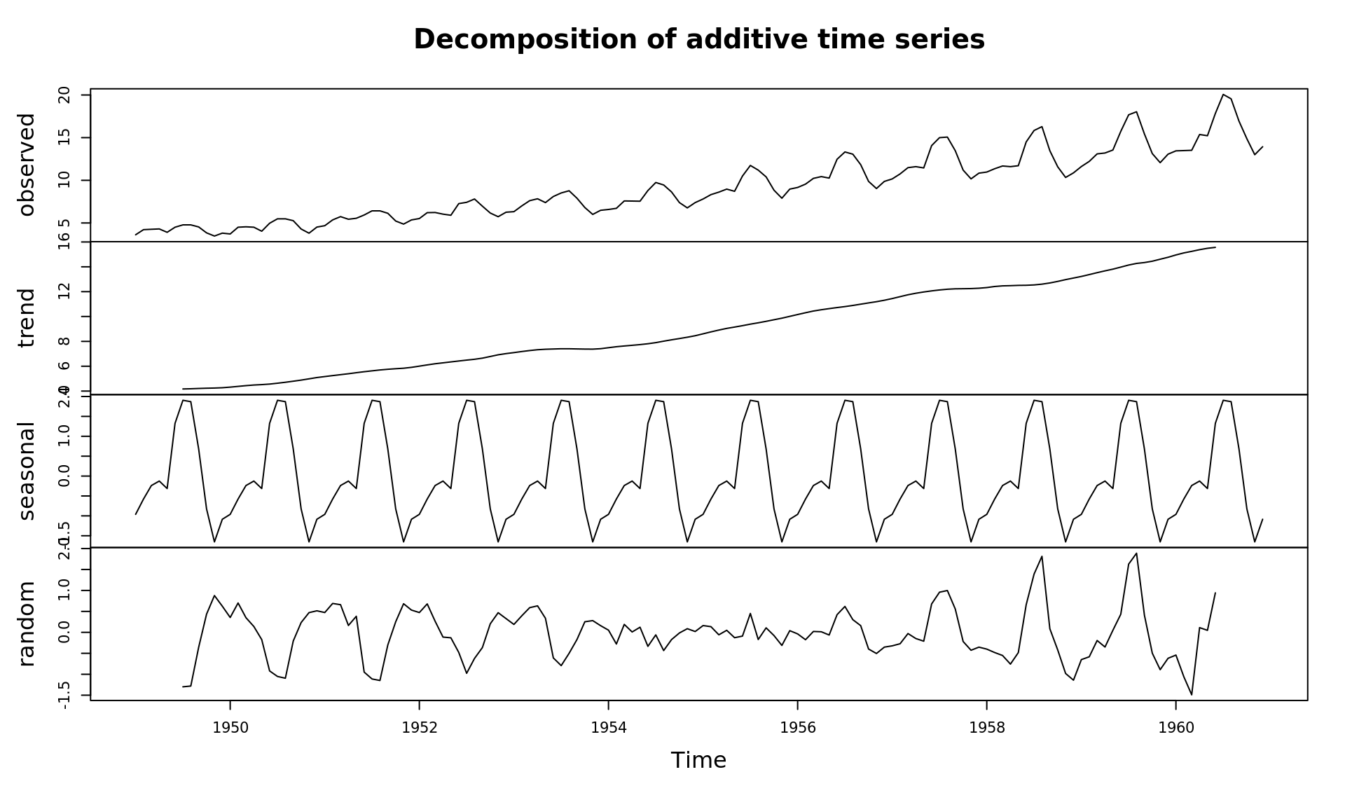
## Decompose average monthly passengers
plot(decompose(Air$month.avg))

## Decompose average monthly passenegers under Box Cox
## Results better random error
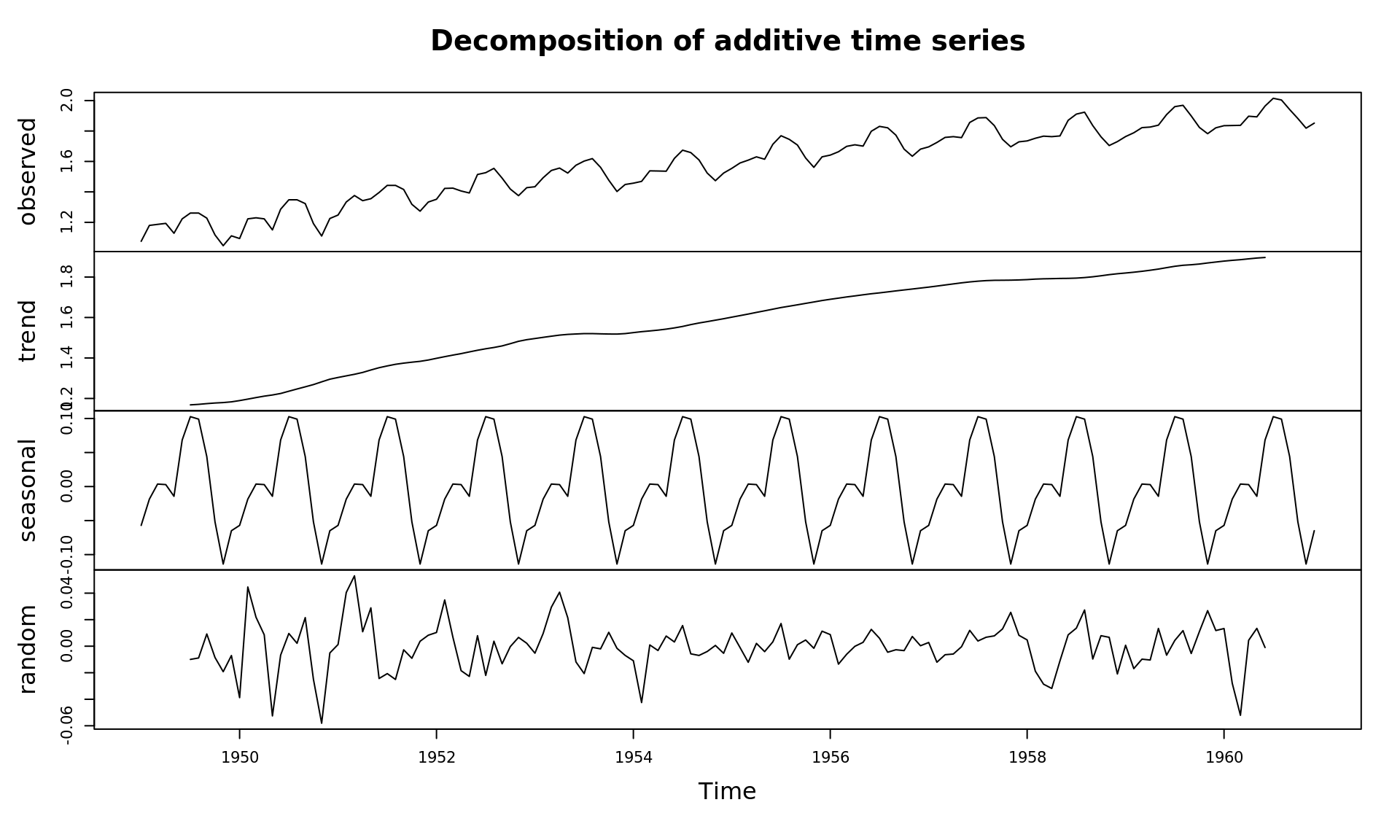
plot(decompose(BoxCox(Air$month.avg, BoxCox.lambda(Air$month.avg))), ylab = "Passengers")